How to merge rows in Excel 2010 and 2013 without losing data

This tutorial provides solutions for 4 different scenarios of merging rows in Excel. See how you can quickly merge multiple rows without losing data; combine duplicate rows, repeatedly merge blocks of rows and consolidate matching rows from two different spreadsheets.

Merging rows in Excel is one of the most common tasks that all of us need to perform every now and then. The problem is that Microsoft Excel does not provide any decent tool to do this. For example, if you try to combine two or more rows in your worksheet using the Merge & Centerbutton (Home tab > Alignment group), all you'll get is the following error message:

"The selection contains multiple data values. Merging into one cell will keep the upper-left most data only."

If you click OK, the merged cells will contain only the value of the top-left cell, all other data will be gone. So, obviously we need to come up with some other solution. And further on this this article you will find several methods that will let you merge multiple rows in Excel without losing any data.

• How to merge rows in Excel 2010, 2013 and 2016
• How to combine duplicate rows (with unique data only)
• How to repeatedly merge blocks of rows in Excel
• How to combine matching rows from 2 spreadsheets

How to merge rows in Excel without losing data

The task: you have a customer database where each row contains certain details such as the product name, product key, customer name and so on. What we want is to combine all the rows related to a particular order, so that the result would look similar to this:

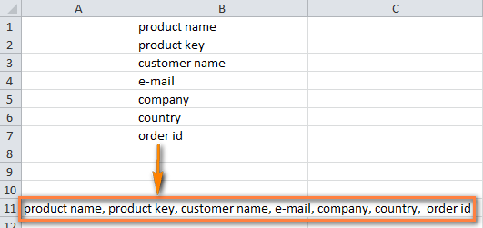
When it comes to merging Excel rows, there are two ways to achieve the desired result:

• Merge Excel rows using a formula
• Combine multiple rows using the Merge Cells add-in

How to merge multiple rows using Excel formulas

Microsoft Excel provides several formulas that can help you combine data from different rows. Probably the easiest one to use the CONCATENATE function. Here are a few examples to concatenate several rows into one:

• Merge rows and separate the values with comma: =CONCATENATE(A1,", ",A2,", ",A3)
• Merge rows with spaces between the data: =CONCATENATE(A1," ",A2," ",A3)
• Combine rows without spaces between the values: =CONCATENATE(A1,A2,A3)

I believe you have already deduced the general rule to write such a formula - simply enter all cells to be merged separated with commas, and then type the separator in between, e.g. ", " is a comma with a space; " " is only a space.

So, let's see how the CONCATENATE formula will work on the real data.

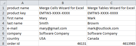
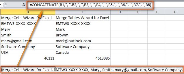
1. Select an empty cell on the sheet and enter the formula into it. We have 9 rows of data, so the formula is going to be pretty large: =CONCATENATE(A1,", ",A2,", ",A3,", ",A4,", ",A5,", ",A6,", ",A7,", ",A8)
2. Copy the formula across all other cells in the row, the result should look similar to this:
   
3. Now you have several rows of data merged into one row. But your combined rows are, in fact, formulas and if you want to convert them to values, you can simply copy / paste the merged rows to some other row in your spreadsheet. The following tutorial explains how to do this in detail: How to replace formulas with their values in Excel.

How to combine rows in Excel using the Merge Cells add-in

The Merge Cells add-in is purposed for combining various types of cells in Excel. It merges individual cells as well as combines data from entire rows or columns. This is how the Merge Cells button looks like on the Excel Ribbon:

To merge two or more rows in your table, proceed with the following 4 steps:

1. Select the rows you want to merge and click on the Merge Cells icon.
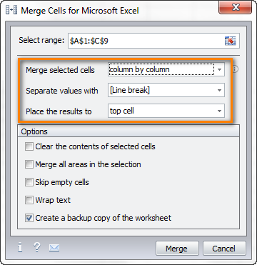
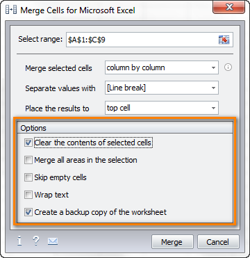
2. The Merge Cells dialog window will open with your table or range already selected, as you can see in the screenshot below. In the upper part of the window, you specify three basic things:
   • How you want to join cells. To merge rows of data, select "column by column".
   • How to separate the merged values. There is an array of standard separators to choose from: comma, space, semicolon and even line break! If you want to use some other separator, merely type it directly in this field.
   • Where to place the merged cells. This can be either the top cell or bottom cell.
   
3. Now let's have a quick look at the lower part of the window to see if you need any aditional options:
   • Clear the content of selected cells. Select it if you want the data to remain in the merged cells only.
   • Merge all areas in the selection. This option will let you merge rows in two or more non-adjacent ranges.
   • Skip empty cells and Wrap text. These two are self-explanatory, aren't they?
   • And finally, you see the "Create a backup copy of the worksheet" option, checked by default. This is just a precaution that will keep you on the safe side and ensure that you won't lose your data in any case.
   
4. Now let us click the Merge button and see what we get as a result - perfectly merged rows of data separated with line breaks!
   

You can download a fully-functional trial version of Merge Cells addin now, try it on your own data and see if it's the right tool for you. The add-in works with all versions of Excel 2016, 2013, 2010and 2007.

How to combine duplicate rows into one (keeping unique values only)

The task: you have some Excel database with a few thousand entries. A bunch of values in one of the columns are essentially the same while data in other columns are different. What you'd like to have is combine data from duplicate rows based on a certain column, making it a comma separated list. Additionally, you may want to merge unique values only, omitting duplicates and skipping empty cells.

The screenshot below illustrates what we are trying to achieve.

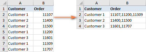
Finding and merging duplicate rows in Excel may be a real nightmare and obviously everyone would like to avoid doing this work manually. In this case, another add-in, Combine Rows Wizard, may come in truly handy.

As I've said, combining duplicate rows in Excel seems to be a pretty tricky task, but the Combine Rows Wizard will walk you through the process making it really simple. And again, you'll need just 4 quick steps:

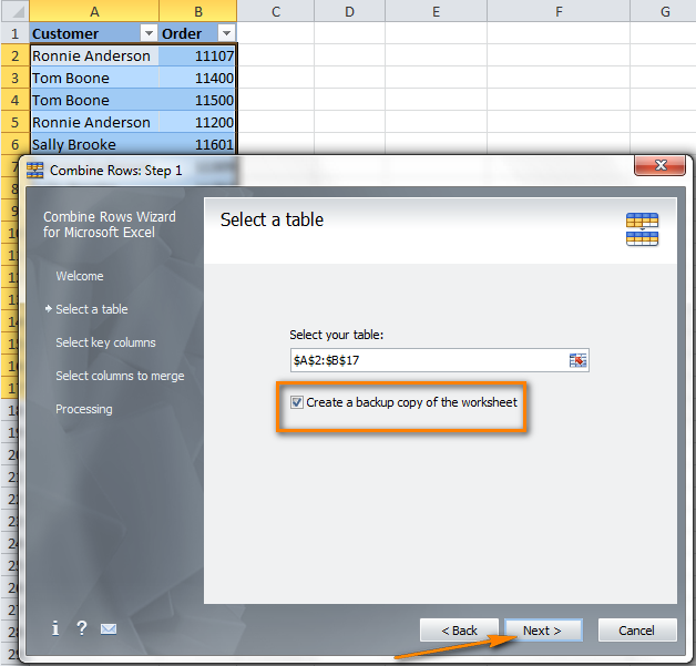
1. Select the duplicate rows you want to merge and click the Combine Rows Wizard icon on the ribbon. Make sure the "Create a backup copy" option is checked, especially if you are using this add-in for the first time.
   
2. Select the key column. In our example, we're selecting the "Customer" column (A) because we want to combine rows based on customer name. If you want to skip empty cells, be sure to select this option in the upper-right corner and click Next.
   
3. Choose the columns to merge. On this step you select the columns whose data that you want to combine and specify the delimiter: semicolon, comma, space, line break or any other character(s) of your choosing. Two additional options in the upper part of the window let you:
   • Delete duplicate values while combining the rows, and
   • Skip empty cells.
   
4. Click the Finish button and you'll see the result in a moment.
   

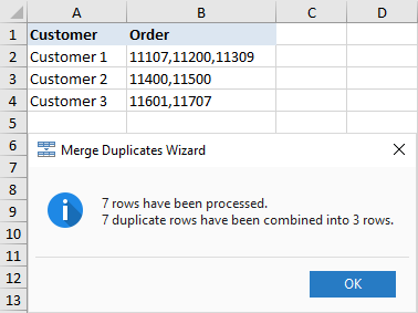
That was pretty easy, isn't it? To make sure of this, go ahead and download the trial version of Combine Rows add-in. You can use it with any version of Excel 2016, 2013, 2010 and 2007.

Repeatedly merge blocks of rows into one row

The task: you have an Excel file with information about the recent orders and each order takes 3 lines: product name, customer name and date of purchase. What you need is to merge every three rows into one, i.e. repeatedly merge the blocks of three rows in an Excel sheet.

This is what we are looking for:

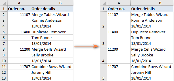
If you have a fairly few entries to be combined, you can select each 3 rows and merge each block individually using the Merge Cells Wizard as we discussed in How to merge Excel rows without losing data. But if you have hundreds and thousands of records in your database, this is definitely not a very elegant solution. There is a quicker way to achieve the needed result:

1. Create an additional column in your worksheet; it is column C in our example. Let's name itBlock Id, or maybe you can come up with a more meaningful name : )
2. Write the following formula to the 2^nd cell of that column (C2) because most likely your table has headers: =INT((ROW(C2)-2)/3). And then copy it across the entire column.
   Now, what does this formula actually do? It adds a unique number to each block of rows to be merged, as shown in the screenshot:
   
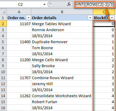   In more detail, the INT function in Excel is used to round a number downwards to the next lowest integer. (C2)-2 deducts the row number where your data start, for the formula to start counting from zero.  For example, our data start from the 2^nd row, so we deduct 2. If your data (actual data, not table headers) start, say, from row 5 and you enter the formula in cell D5, then you put (D5)-5. And finally, we divide by the number of rows to be merged in each block (since we are combining the blocks of three rows, we add /3 at the end of the formula). Phew, I do hope my explanation makes sense. If not, don't hesitate to ask in comments and I'll try to come up with something easier to comprehend : )
3. Well, the previous step actually did the main part of the work. Now you just need to merge the rows based on column Block Id using the Combine Rows Wizard, exactly in the same way as we did in the previous example when combining duplicate rows.
   
   And here's what we have as the result:
   
4. Delete the Block ID column since you don't need it any longer and you are done! Funny enough, that we've needed 4 steps again, like in two previous examples : )

Merge matching rows from 2 Excel worksheets without copying / pasting

Task: you need to merge rows from 2 tables based on a common column. The tables may be located in the same sheet, in two different spreadsheets or even in two different workbooks. For example, you have sales reports for January and February in two different worksheets and you want to combine them into one.

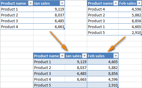
Mind you, each workbook may have a different number of records and different order of product names, so you cannot simply copy and paste the "Feb Sales" column to the first workbook because the products won't match.

Another add-in from AbleBits will work a treat in this case - Merge Tables Wizard. This tool will find, match and merge rows from two Excel worksheets in seconds, no matter how many rows each spreadsheet contains. The design of the wizard is pretty much similar to the Combine Rows Wizard we've used in two previous examples, so it should already look familiar to you : ) Okay, to combine matching rows from 2 spreadsheets, do as follows:

1. Select the 1st table, this is the main table that you want to update, and click the Merge Tables button on the Ribbon (Ablebits Data > Merge).
   
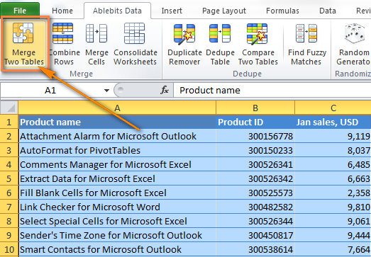   This will open the Merge Tables Wizard's dialog with your first table already selected, so simply click Next.
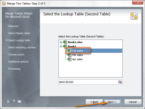
2. Select the second worksheet, i.e. a lookup table where you want to search for matching rows.
   
3. Choose the column with unique values that exists in both tables, it will be used as a unique identifier. It our example, it can be either Product Name or Product ID, or both.
   
   You can also click the Auto Detect button at the bottom left-hand corner and the wizard will find the key column(s) automatically.
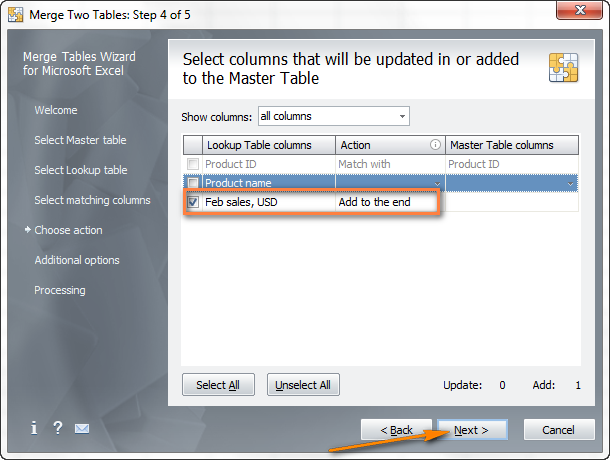
4. Choose which column(s) you want to update and which add to the end of the 1^st table. Since we want to add only the "Feb sales" column, let's select it and click Next.
   
5. On the next step, the Merge Tables Wizard provides a few additional options, such as:
   • Add non-matching rows to the end of the table
   • Update only empty cells in the main table
   • Highlight updated rows in a color of your choosing
   Actually, there are some more options, as you can see in the screenshot below: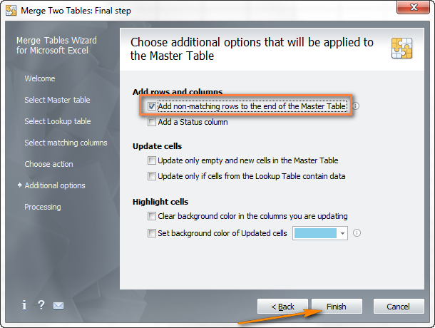
   
   If you don't need any of these options for now, you can skip this step and click the Finishbutton.
   However, if your second worksheet may contain some rows that do not exist in the first spreadsheet and you do want to add them, select Add non-matching rows to the end of the table.

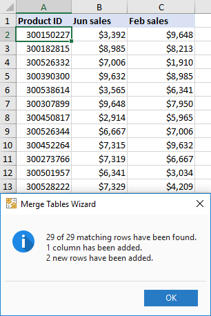
Now click Finish, wait for a couple of seconds and as the result you have all matching rows from two Excel worksheets merged into a single table:

If you are interested to try the Merge Tables Wizard, go ahead and download a trial version here. As well as the two previous tools, it support Microsoft Excel 2016 - 2007.

Share :

Tweet

✚

Related Post